# Per-block-group race shares — one row per BG, with stage flags.
# bg_pct_white_2013 / bg_pct_black_2013 are already on a 0-100 scale.
bgs_at_stage <- value_df |>
filter(!is.na(bg_geoid)) |>
group_by(bg_geoid) |>
summarise(
pct_white = dplyr::first(bg_pct_white_2013),
pct_black = dplyr::first(bg_pct_black_2013),
s1 = any(reach1, na.rm = TRUE),
s3 = any(reach3, na.rm = TRUE),
s4 = any(reach4, na.rm = TRUE),
s5 = any(reach5, na.rm = TRUE),
.groups = "drop"
)
fig4_hist_data <- bgs_at_stage |>
tidyr::pivot_longer(c(s1, s3, s4, s5),
names_to = "stage_key", values_to = "in_stage") |>
filter(in_stage) |>
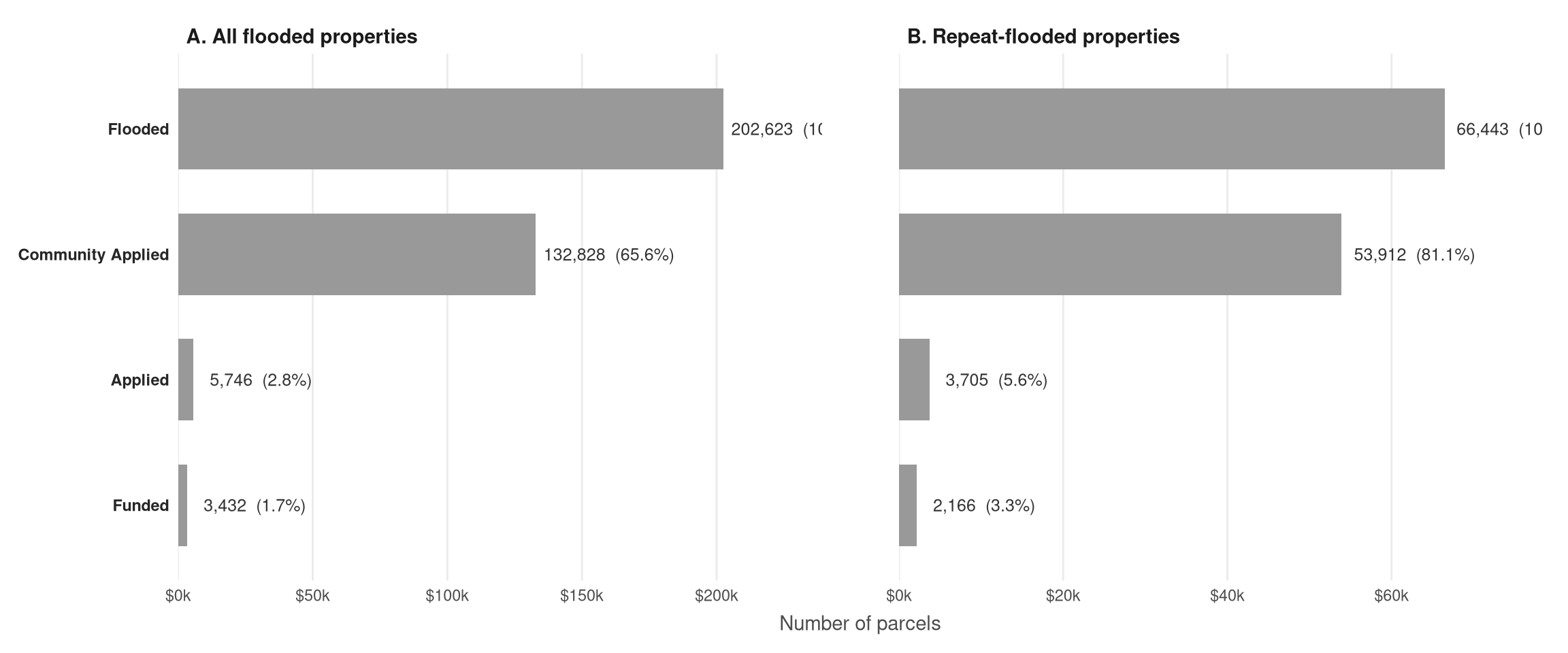
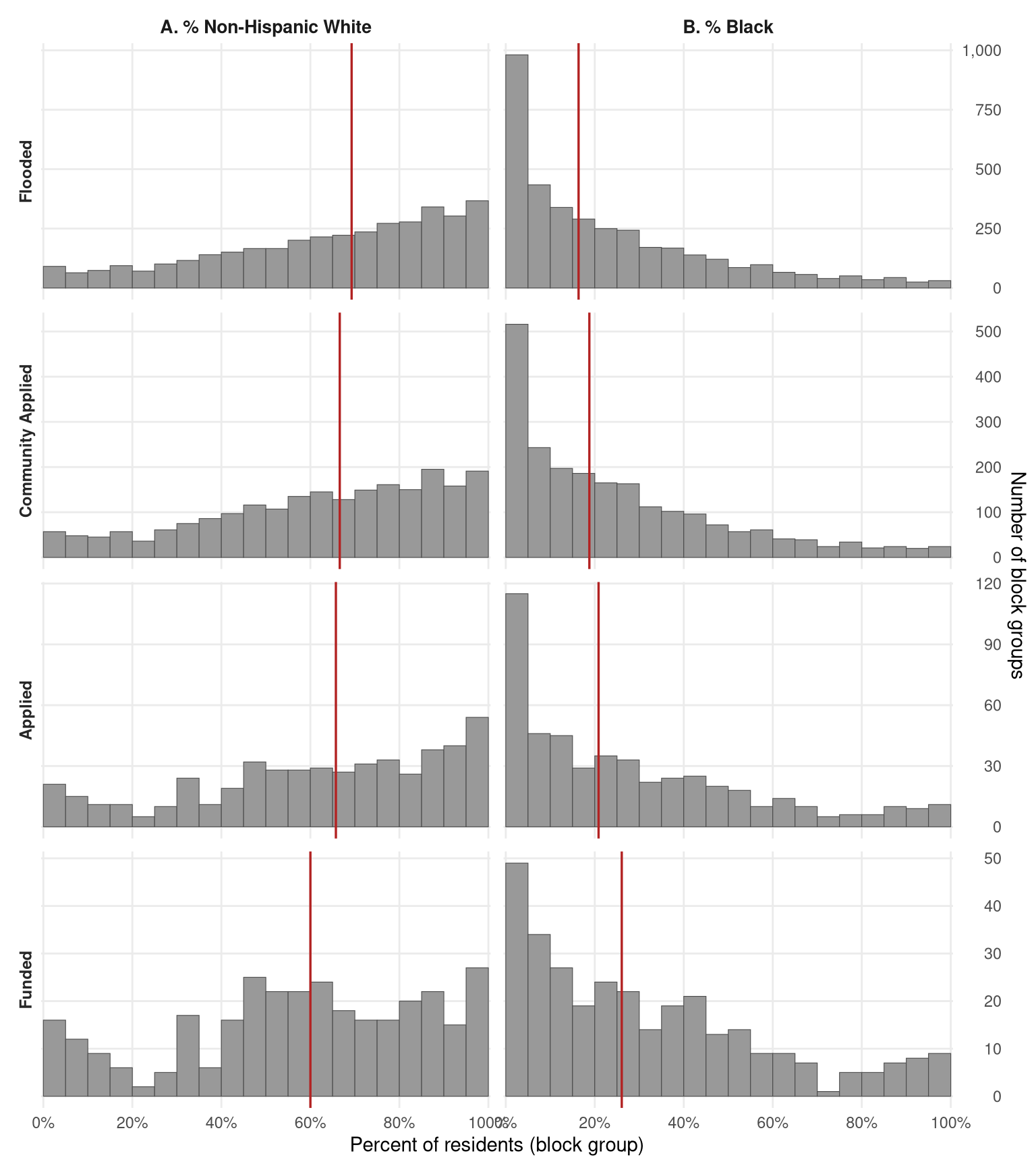
mutate(stage = recode(stage_key,
s1 = "Flooded", s3 = "Community Applied",
s4 = "Applied", s5 = "Funded"
)) |>
select(stage, pct_white, pct_black) |>
tidyr::pivot_longer(c(pct_white, pct_black),
names_to = "race", values_to = "pct") |>
filter(!is.na(pct)) |>
mutate(
stage = factor(stage, levels = stage_levels_4),
race = factor(recode(race,
pct_white = "A. % Non-Hispanic White",
pct_black = "B. % Black"
), levels = c("A. % Non-Hispanic White", "B. % Black"))
)
fig4_medians <- fig4_hist_data |>
group_by(stage, race) |>
summarise(median_pct = median(pct, na.rm = TRUE), .groups = "drop")
fig4 <- ggplot(fig4_hist_data, aes(x = pct)) +
geom_histogram(binwidth = 5, boundary = 0,
fill = "grey60", colour = "grey30", linewidth = 0.2) +
geom_vline(data = fig4_medians,
aes(xintercept = median_pct),
colour = "firebrick", linewidth = 0.6) +
facet_grid(stage ~ race, scales = "free_y", switch = "y") +
scale_x_continuous(limits = c(0, 100), breaks = seq(0, 100, 20),
labels = function(x) paste0(x, "%"),
expand = c(0.005, 0)) +
scale_y_continuous(position = "right",
labels = scales::label_comma()) +
labs(
#title = "Fig. 4 Neighborhood racial composition by HMA stage",
#subtitle = "Census block groups, 2013 ACS",
x = "Percent of residents (block group)",
y = "Number of block groups"
) +
theme_minimal(base_size = 11) +
theme(
strip.text.x = element_text(face = "bold", size = 10),
strip.text.y.left = element_text(face = "bold", size = 9, angle = 90,
hjust = 0.5, colour = "grey15"),
strip.background = element_blank(),
strip.placement = "outside",
panel.grid.minor = element_blank(),
panel.spacing = unit(0.5, "lines"),
plot.title = element_text(face = "bold")
)
fig4